Economics of Home Ownership Deep Dive

Evaluating home purchase scenarios and associated investment opportunity costs.

Photo by Breno Assis on Unsplash.

Part 1 of Home Purchase Scenario Model Analyses.

Introduction.

For those who have previously considered or are considering the purchase of a home, then this post is meant for you to help customize your scenarios and vet your available options. I hope that you find the included financial model, available here, informative as you evaluate potential home purchase scenarios. This post and model should help you understand the full costs associated with home ownership and the inherent opportunity costs of not investing downpayment and ongoing maintenance costs in other assets, e.g., passive market ETFs.

Given my avid interest in investing and the fact that my wife and I purchased a home in 2018, I recently revised my approach to modeling out our monthly expenses, long-term savings plan and forecasting additional funds we’ll have to allocate to our family’s investment strategies. Also, with the enduring Covid-19 situation, this topic is timely since more millennials are now considering home ownership. This is largely due to the evolving viewpoints many have experienced based on shelter-in-place requirements, the projected migrations out of major cities to suburbs/residential areas and the increasing desire for things many homes afford, such as a yard and better WFH office space.

In this post I provide context and a scenario-based model that you can use to evaluate different home purchase options, including variable purchase prices, down payment amounts, and lending terms, among several others. The scenario-based model has flexible inputs, allowing you to customize it based on your current income(s), monthly expenses, and your personal financial situation and investment preferences.

Please note that this model does not yet account for all considerations, such as 1) whether or not you should refinance and how to evaluate multiple options there, 2) it doesn’t present a full rent versus buy analysis (I link to a helpful resource and it does factor in net recurring costs in the home ownership IRR), 3) evaluates 15 and 30 year fixed but not other loan types, e.g., ARM and 4) it doesn’t account for taking on PMI (lower than 20% downpayment) and eliminating PMI once loan-to-value becomes <= 80%. In true product management fashion, I’ll iterate on future posts if there’s enough interest for features like this.

Personal pain point and reason for building this scenario-based model. While there are a number of useful online resources that can help inform your home purchasing decision, some of which I’ll share in a bit, where I believe this post is unique is that it will take those analyses several steps further and can be personalized to your decision set. In this initial post, I’ll share a framework for how to evaluate different home purchases; and this framework will also assist you in thinking through the associated opportunity costs you’ll encounter when tying up equity in a home versus other potential investments. In other words, given your personal assumptions, it’ll help you forecast out what the money you didn’t put into a larger home would have returned in the market (or some other asset of your choice); and whether or not you’re better off with the home scenario you selected versus investing your capital elsewhere. I have not found another resource that provides this personalized evaluation as part of a home ownership scenario analysis.

In a follow-up that I will complete based on interest in this post, my plan is to turn again to Mode Analytics (older example here). In part 2, you’d further your data science analytics and dashboard development skills, creating an interactive dashboard that charts the various scenarios your financial model generates given your personalized inputs. The model, for that future post, would generate a CSV file that can be used as a flat file data source for an interactive Mode Analytics dashboard.

In tandem with this post, my other related articles that talk further about establishing an investment system by leveraging Python include:

1. Part 1: Extract financial time series data from Yahoo! Finance API in Jupyter notebook
2. Part 2: Extend Part 1’s analyses and visualizations by providing the code needed to take the data sets generated and visualize them in a Dash by Plotly (Dash) web app
3. Part 3: Build on the Stock Portfolio Analyses and Dash by Plotly approaches to understand your total shareholder return (TSR) and track Robo Advisor-like Portfolios.

Disclosure: Nothing in this post should be considered investment advice. Past performance is not necessarily indicative of future returns. I am writing about generalized examples and show how to evaluate home purchase scenarios and the relative opportunity cost to allocating some/all of this capital to other investment opportunities. You should direct all investment related questions that you have to your financial advisor and perform your own due diligence on any investments mentioned in this post. Therefore, I assume no liability for any losses that may be sustained by the use of the method described in this post, and any such liability is hereby expressly disclaimed.

Becoming Smarter on Home Ownership Economics.

As mentioned in the intro, there are four limitations (I’m aware of) to my approach: 1) does not evaluate refinancings, 2) no full rent versus buy analysis, 3) looks exclusively at fixed rate mortgages (e.g., 15 and 30 year) and 4) model doesn’t account for PMI scenarios. Below I share resources that address #s 1 and 2. If #4 becomes of interest based on feedback, then I’ll look to update the model to evaluate. My personal situation has not involved PMI as I’ve always considered a house where I was able to put down 20%+. This decision is personal and if people need additional guidance here for PMI related scenarios, I’m happy to re-evaluate.

Refinance evaluations. I really enjoy Zillow’s tools across the board and have found their refinancing calculator to be helpful, at a high level, as I’ve evaluated potential refinancings. As general guidance, the short form rule of thumb is to understand what your closing costs are, aka what are you being charged to complete the refinancing; let’s say those are $2k. Then look at your monthly savings versus current monthly payment; let’s say that’s $100 per month. This means it would take you ~20 months ($2k / $100 per month) to earn back your upfront costs on the refinancing. Needless to say, you should stay in your house for more than 20 months for this to start to make sense.

Rent versus Buy. In considering the rent versus buy evaluation, I believe Travis Devitt put together a helpful resource on this, which formed some of my thinking and helped me be much smarter about the considerations here: link to Travis’s tweet.

Resources. Before you get started with the model in this post, I’d encourage you to read through the first two resources below to have a much better understanding of the economics of home ownership. Of note, the Betterment post is extremely detailed and helpful; I’ve based several of my model’s base case assumptions using data directly from this post. The last resource presents data and addresses head on the homeownership gap that persists in America. I’m unfortunately not an expert and do not have all of the answers, but I’m more than willing to contribute to causes and provide help/answers where I can to support closing this gap. Please feel free to reach out to me on Twitter, @kevinboller, or leave a response to this post, if there’s a cause you recommend I look into or a question that I can help answer on the homeownership topic covered in this post.

1. Wealthfront Home Planning Guide.
2. Betterment - is buying a home a good investment?.
3. Article on home ownership gap in America..

Using the Scenario-based model.

Inputs worksheet.

When you open up the model, you will start on the Inputs worksheet that drives the rest of the formulas throughout. The schedule on the Monthly Model sheet provides a 10-year forecast. You can certainly extend this further if you would like, but it’s hard for me to believe that the average person is making a 30-year decision and I prefer to evaluate shorter time periods; this is particularly because all models are wrong and trying to model out the next 30 years is likely even more wrong than the next 10.

Cell C2 on the Inputs sheet is the most important cell in the entire model. Everything in column C on this sheet should also not be modified, as the inputs will fill in based on the selected scenario, chosen in C2, which pulls from column 1 to n columns away from column C. In the columns to the right of column C, and you can add more scenarios to the right if you’d like, you change the assumptions based on your particular scenarios that you’re evaluating. Note that any cells in blue font mean that they can be modified, and any cells in black font should not be since they’re formula based and are scenario agnostic. While these scenarios are all positive cases, e.g., 3.2% home appreciation, you can certainly evaluate the same scenario multiple different ways. For example, maybe you want to compare a base scenario of 3.2% growth and 7% investment returns versus 0% housing appreciation and 4% investment growth to see the impact over time to your adjusted net worth.

Key point: always be cognizant that when you make any adjustments to scenarios 1 - 4, you should always go back and cycle through the scenarios in cell C2 - type 1, 2, 3, 4 into C2 in order to cycle through these scenarios and have their inputs flow through the model; this will become evident once you get use to the remaining worksheets.

The Home Purchase Details and Loan Details sections, if you’ve read the resources noted above, should be straightforward. In columns D - G, I’ve included 4 templated scenarios. The Income and Expenses have placeholder values and should be adjusted to reflect your personal income and expenses. I would put in after-tax income figures, so that you have a better estimated proxy for what your cash flow will be after servicing your monthly expenses; and the capital that you’ll have available to invest after those expenses are serviced. For the remaining expenses after HOA, such as home maintenance, I’d recommend leaving those as is since they’re based on the Betterment post’s data. Same recommendation for the Home Sale Inputs assumptions, including selling and closing costs.

For the Investment Performance, % of excess cash invested means that, for the money you retain post paying your monthly expenses, how much of that will you invest into a passive ETF, etc. You then must make an estimate on your nominal return, which I’ve set at 7%. You can choose to be more/less aggressive than this. Your available cash reserve, which you likely would not need, is money set aside in the event that you need more cash to support expenses in a given month (expenses exceed income); you might do this if your monthly expenses exceed your income but you manage cash flow during the year anticipating lumpier cash inflows, e.g., RSU vests twice per year; but this is not necessarily advisable or applicable to most.

Net Worth Inputs, the last section, is how you’ll directly compare your home investment and other investments across scenarios to see the impact on your net worth. Again, the annual home appreciation of 3.2% is a Betterment post assumption. The down payment opportunity cost means, in scenarios where you pay a larger down payment than the base scenario (always have base in column D), we’ll deduct what that capital would’ve returned if invested elsewhere (instead of used for a larger down payment). Since the extra downpayment upside is reflected in the return of the home value in the scenario where you buy a larger home and/or pay more upfront, this will show your net return relative to base. It should also make all scenarios apples-to-apples when comparing the base with scenarios that have higher upfront home costs.

Monthly Model worksheet.

In cell C1, you’ll see the current scenario being evaluated based on the scenario you’ve input into C2 on the Inputs worksheet. This model shows a monthly breakdown across 10 years, and also rolls these up to annual totals for those 10 years. Row 37 shows net operating profit pre-tax, which takes your post tax income and deducts your monthly expenses. While I recommend income to be entered post-tax, the spreadsheet cannot account for your actual tax scenario; therefore I’ve called it pre-tax as further adjustments will occur when you file/pay taxes. Below this is your debt paydown (rows 45-49) and a schedule that goes through what excess cash will be invested, the projected returns from those investments, and the cash reserve (money not invested) that will build over time.

You’ll see in rows 65-67 the buildup of your investable cash over time. For relevant higher cost scenarios, the opportunity cost for what you could have returned by buying a smaller home/making a smaller down payment will also accrue value over time in the same manner. It’s important to note that the investment returns in this model offer a simplified, linear view of your money growing over time. No investment will grow linearly at your annual expected return divided by 12 months; further, since this is exhibiting a dollar cost averaging approach, where you invest when you have available capital on a monthly basis, your returns will exhibit more volatility than the simplified model framework. Regardless, you shouldn’t get bogged down in the monthly returns and recognize that 1) you will, on average, see this appreciation annually in your investable assets (home and ETFs, et al) and 2) this model is intended to help you take a longer-term view. Ideally, given the friction in transaction and closing costs, you’ll provide yourself with 5 to 10 years in your home before deciding on moving/buying a different home.

Net Worth over Time first evaluates the build up in home equity. This is driven off the input to annual home appreciation (which is adjusted to a monthly rate of increase in Inputs) and the paydown in debt based on the terms of the mortgage. To finalize the net worth calculation, the upside the additional down payment would’ve generated in scenarios beyond base scenario is deducted, investment growth is added and you can manually input any additional assets and liabilities that you’d like. My personal model schedule is more detailed than this, including retirement assets (Roth, 401k, etc.). You likely want to build those into your model if you’d like a complete picture of your net worth alongside the projected contributions to those accounts and related growth over time.

While home equity grows over time, increasing your overall net worth, the Betterment article does a good job of highlighting the “problems with calculating investment returns”. For sake of brevity, there are three core drivers, in addition to home appreciation, that impact your return on home investment: 1) transaction costs, 2) cash flows, including ongoing costs (note, these are reflected in our model, see row 49 on Inputs worksheet), and leverage, aka a mortgage, increasing gains to the upside but also increasing risk on the downside. As a result, to see a true apples-to-apples comparison, in the Charts and the Recurring Costs + IRR worksheets, we’ll see how you’ll need to deduct estimated transaction costs in order to reflect your true net worth and your home investment’s projected IRR.

Charts worksheet.

On the Charts worksheet, we compare a few core metrics across scenarios over the first 5 year period. Extending this to 10 years, or beyond if you extend the model further, should be straightforward if you have some familiarity with developing and extending models.

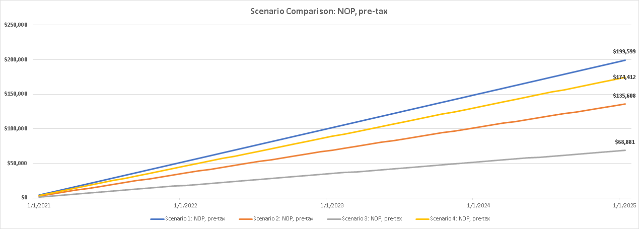
In the first chart, we compare your projected net operating profit (NOP, income less expenses) across scenarios. You can see in this case that NOP is greatest in scenario 1 and second highest in scenario 4. In scenario 4, you’ve elected to pay for the same home as scenario 1, but you’ve selected a 15-year mortgage over a 30-year one. To each their own, but I subscribe to Ric Edelman’s theory of having a 30-year mortgage. - I prefer greater liquidity and diversification. Using these scenarios, you can see in Scenario 2 that you’ll have ~70% of the NOP you have in scenario 1, and in Scenario 3 you have ~35% of the NOP you would’ve had in Scenario 1 (in this scenario, you bought a home 3x as expensive as Scenario 1).

In the second chart, go to cell K101, the chart shows investment details for the selected scenario, and the table below breaks down the scenarios head to head. Given the linearity of returns and the same assumptions regarding how much is invested (80%), you’ll see that your total investment balance + excess cash for the scenarios past #1 will mirror the differences in NOP between scenarios. You can decide if you’d like to modify the scenarios’ assumptions; for example, if you buy a smaller home, maybe you’ll allocate more of your capital to investing (90%?) and/or be more aggressive with your other investments, expecting a return higher than 7%.

In the 3rd chart, go to J160, you’ll see your net worth over time and your debt paydown over time on the secondary y-axis. For the first three scenarios, the existing loan balance as a % of original mortgage, and home equity as a part of home valuation are relatively in-line. The only difference is that I’ve assumed modestly higher interest rates for larger home purchases/greater amount borrowed. You’ll also see that your equity reflects 30% of your net worth in scenario 1, increasing to ~60% and 90%+ in scenarios 2 and 3, and arriving at 40% in scenario 4 (where you’ve elected a 15-year mortgage; higher than scenario 1 given this). While you might conclude in column O (cell 0160) that you’re indifferent across scenarios and your net worth is relatively the same, this is not entirely correct. After deducting for projected closing costs (see U161), which estimates the net realized value you could get from the sale of your home, you see that, after 5 years, scenarios 2 and 3 actually trail scenario 1 for your adjusted net worth; whereas you’re effectively in the same spot in scenarios 1 and 4 (same purchase, different mortgage duration). The near tie between scenarios 1 and 4 indicates that, based on your investment opportunity set, you’re relatively indifferent to investing more in your home (shorter duration mortgage) versus in a diversified ETF (assuming a 7% annualized return). For final details on how to evaluate your potential home investment’s returns, we’ll go to our last worksheet.

Recurring Costs + IRR worksheet.

As stated a few times now, the Betterment article is well detailed and very helpful to become more knowledgeable on the mechanics and implications of home ownership. However, after reading the article, you’ll still not have a way to customize the learnings to your personal situation or decision set. Given that I agreed much with the author’s approach to returns, I’ve re-created two of the tables in that post within my last worksheet. The benefit is that you’ll be able to tweak scenarios and inputs and they’ll flow through these tables based on the same structure as that post.

In the Annual Recurring Costs of Home Ownership table, this lays out how to calculate net annual recurring costs (rent versus buy) for the particular scenario that you’re evaluating. For detail on this, see Ongoing Costs of Home Ownership in the Betterment post. Since this may raise questions, I’ll point out a difference between the model in my post and the table from the Betterment one. In the Betterment table, annual property taxes grow with the value of the home and homeowner’s insurance grows at inflation. While this is indeed more accurate, I’ve left each scenario’s fully loaded monthly mortgage payment (including property taxes and insurance) constant over the model’s 10 year forecast. This is to reduce cognitive overload for what we’re covering and to make it easier to understand this model relative to online mortgage calculators. Since I do not grow property taxes and insurance modestly over time, this makes the homeownership returns slightly overstated; however, since this is done equally across scenarios, I believe this has an immaterial impact on your evaluation. To highlight the difference, you’ll notice in the Betterment post’s Annual Recurring Costs Of Homeownership table that, after 10 years, annual property taxes and home insurance costs on a $250k home purchase only increase by ~$500 and $200, respectively.

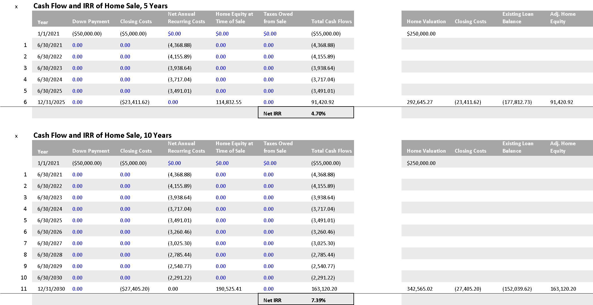
I also show two IRR schedules, one for a five year investment horizon and the other for a ten year investment horizon. You’ll notice that the IRR is highest for scenario 4, where you pay the lowest upfront down payment (same as scenario 1) and you pay down your loan faster due to having a 15-year versus a 30-year mortgage. In this case, while your net annual recurring costs are higher in scenario 4 versus scenario 1, the greater equity value you’ve generated through paying down more of the debt principal drives the higher IRR. This exhibits the upside of the levered return that is home ownership when you benefit from home value appreciation.

However, I’ve simplified some things in the annual recurring costs table, such as the annual rent saved assumption. The annual rent saved should likely be the same for all of your personalized scenarios (please feel free to reflect this in your own evaluation), but given my assumption to drive off of the mortgage payment, saved rent is actually higher in scenario 4 and the other higher cost scenarios. I’ll need to think if this can be represented differently, but the result is that scenario 4’s IRR is likely overstated. For now, I’ve left these tables as more of a generalized illustration of the return profiles across scenarios. If you would like, it should be very easy to override the formulas in columns H and I in the first table on Recurring Costs + IRR. You can just input your particular rent saved and renters insurance saved, and then grow these at inflation.

As expected, Scenarios 2 and 3 have modestly lower IRRs than Scenario 1, since you see the same price appreciation as in Scenario 1, slightly slower debt paydown due to greater interest costs and your net annual recurring costs are higher given the higher mortgage payments. Last, similar to the Betterment post, you see that the returns improve over a longer holding period (10 years versus 5), as it takes time to recoup your upfront closing costs from purchasing the home.

I’d finally note that this model does not present an overall returns analysis across your entire set of assets; and the home ownership IRR is done independently on the final worksheet. My advice here is to focus less on returns but on the outcome that generates the highest adjusted net worth, while balancing the risk you’re comfortable taking to achieve this adjusted net worth. This is a more complicated topic and I’ll consider following up more on this if there is related feedback and questions.

Conclusion.

To conclude this post, I hope that you find this framework useful in evaluating your personal opportunity set in terms of potential homes to buy, related purchase prices and key variables such as % down payment, mortgage interest rates and loan duration. While I’ve pointed to very helpful resources that I found to better understand the economics of home ownership, I’ve not found another resource that 1) personalizes monthly cash flows, 2) forecasts your build up of net worth over time, including home equity, and 3) provides a customized schedule to evaluate potential investment returns and your home’s potential IRR.

The scenarios in this model largely conclude similar findings to those in the Betterment post. It takes on average 4-5 years to break-even on your closing costs, and a home can be a sound investment and have a comparable return profile to a total stock market ETF (such as Vanguard’s VTI).

In combination with the resources I’ve linked to, now that you have a customizable model that allows you to evaluate your decision set across your housing and investment opportunities, you should feel fully informed that you’ll make a well researched decision and step into home ownership with your eyes wide open. In doing so, I believe that owning a home can be a great place to be; and you’ll have a strong grasp on how it fits into your overall personal finances and your forecasted investment and retirement strategy.

If you enjoyed this post, it would be awesome if you would click the “claps” icon (more than once!) to let me know and to help increase circulation of my work. If you would like to leave a comment on any suggested edits, feature requests or interest in a follow-up post, please let me know that as well.

Feel free to also reach out to me on twitter, @kevinboller, and my personal blog can be found here. Thanks for reading!